

Empirical plasmapause model
The PP index based plasmapause model is constructed in two steps. First, a model of the inner boundary of small
scale field aligned currents (SSFACs) is derived as a function of MLT and Kp, then a ‘bulge’ model is added inferred from the observed
difference between the SSFAC boundary and the true plasmapause:
empirical PP model = empirical SSFAC boundary model + bulge model.
The SSFAC boundary
In Fig. 1 the mean positions of the inner boundary of SSFACs calculated from all observations made between 1 Jan, 2014 and 31 March, 2017 from all the three Swarm satellites are presented on a dial plot as a function of MLT at different levels of geomagnetic activity (0≤Kp<1, 1≤Kp<2, 2≤Kp<3, etc.). The detection is restricted to times when the solar zenith angle χ>80°, causing the asymmetric day-night distribution of detections, and the corresponding dayside gap in the boundary. The central half-shaded circle represents the Earth’s sunlit and dark hemispheres. The boundary positions are drawn on the equatorial cut of the magnetosphere. The insert in the bottom right corner presents the MLT distribution of the same boundary crossings. The shape of the boundary in the topside ionosphere is very close to a circle at any level of geomagnetic activity. The size of the boundary, however, is very sensitive to geomagnetic activity, and scales with -Kp. The circles are not geocentric, the centres are shifted somewhat toward noon. The standard deviation of the individual Lssfac observations is also a clear function of Kp, decreasing from ~0.7RE at Kp = 0 to ~0.3RE at Kp = 7, however, it hardly depends on MLT.
Not only the boundary position, but also the boundary width is a function of Kp. The boundary gets narrower when geomagnetic activity increases. At low activity, the mean width is around 3 RE, but the scatter is large, while for Kp>6 it becomes narrower than 1 RE. The overwhelming majority of the boundary observations are made at relatively sharp boundaries, i.e. when the boundary width is lower than 3 RE.
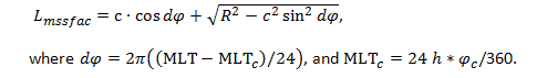
For a given level of Kp, we model the observed boundary in L space by an eccentric circle. The position of a point P on the circle is given by its polar coordinates: Lmssfac and φ=2πMLT/24 as shown in Fig. 2. If the circle is centred at C(c,φc ) and has a radius R, Lmssfac can be derived for any MLT by applying the formula:
 (1)
(1)
Moreover, we suppose, that the position of C and the radius of the circle, R have a linear/quadratic dependence on Kp, respectively, that is
 (2)
(2)
where c0 and MLT0 define the position of the centre and R0 is the radius of the circle both Kp=0, while p1, p2, γc, γmlt are free model parameters. Based on 61512 boundary positions (here χ>90°) observed during the period Jan 1, 2014 - March 31, 2017, the following model parameters (with 95 % confidence bounds) were obtained:

The corresponding model is presented in Fig. 3 as dashed circular curves. The centres of the circulars hardly move with increasing Kp. From Kp = 0 to Kp = 6, it moves from MLTc=11.9, c= 0.18 RE to MLTc=12.9, c= 0.25 RE. The mean residuals (observation - model) in each bin are between -0.3-0.2 RE at all Kp levels between 1 and 6. At Kp = 0 the mean residuals are somewhat larger.
The bulge model
The plasmasphere is well-known to have a dusk-side bulge and its distance at different MLTs can be quite different, controlled by the past variation of magnetospheric convection. On the contrary, the SSFAC boundary responds almost simultaneously at all MLTs (within about an hour) to changing conditions. The two boundaries are coupled only near midnight and in the early morning sector (Heilig and Lühr, 2017).
For calibration, we used NASA Van Allen Probes PP crossings obtained from in-situ electron density observations. We estimated the mean separation between the SSFAC boundary and the PP as a function of MLT. The calibration is based on 1762 Swarm crossings and the simultaneous (UT difference is less than ±1 h) VAP PP observations. The comparison revealed a clear bulge signature in the pre-midnight sector (19-01 h MLT) peaking at 21-22 h MLT. Elsewhere the SSFAC boundary is found typically poleward of the PP by ~0.5 R (Fig. 4). This result is very similar to the obtained differences between CHAMP and IMAGE observations (Heilig and Lühr, 2013). However, for individual cases the location of the boundaries can be very different. While the PP, due to its co-rotation with Earth and the localized erosion, is determined by the Kp evolution of the preceding days, the PP index responses within a few hours simultaneously at all MLTs.
The 'bulge' model is deduced from the difference:
 (3)
(3)
Application of the model
The model derived in the previous section can be used in various ways. First, it can be used as a climatology model. When no boundary observations are available, Lmod can be calculated directly from MLT and Kp as inputs, then the bulge model value corresponding to the MLT in question has to be added. Using the model this way is similar to using any other statistical PP model:
 (4)
(4)
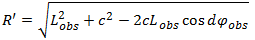
However, the strength of this model is that it can be used in synergy with PP indices, i.e. direct observations. If we have an observation of Lssfac=Lobs at a certain MLTobs and the geomagnetic activity given by the Kp index is known, we can, by combining the model (yielding the shape and the centre of the boundary) with the actual observation (providing the actual radius), estimate Lssfac at any other MLT. This is done by rescaling the size of the boundary based on the actual observation, while taking the average circular shape and the Kp-dependent centre position from the model:
 (5)
(5)
Moreover, since the Kp dependence of both c and MLTc is found to be very weak, we can regard them as constant, e.g. c=0.2 RE, MLTc=12 h, while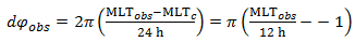 can be calculated from the model. Neglecting the Kp dependence of the centre position will cause less than 0.05 RE error.
Now Lmssfac at any MLT can be computed by the direct use of Eq. (1), but substituting R’ into R. The model PP position is
found again after adding the 'bulge' model.
can be calculated from the model. Neglecting the Kp dependence of the centre position will cause less than 0.05 RE error.
Now Lmssfac at any MLT can be computed by the direct use of Eq. (1), but substituting R’ into R. The model PP position is
found again after adding the 'bulge' model.
empirical PP model = empirical SSFAC boundary model + bulge model.
The SSFAC boundary
In Fig. 1 the mean positions of the inner boundary of SSFACs calculated from all observations made between 1 Jan, 2014 and 31 March, 2017 from all the three Swarm satellites are presented on a dial plot as a function of MLT at different levels of geomagnetic activity (0≤Kp<1, 1≤Kp<2, 2≤Kp<3, etc.). The detection is restricted to times when the solar zenith angle χ>80°, causing the asymmetric day-night distribution of detections, and the corresponding dayside gap in the boundary. The central half-shaded circle represents the Earth’s sunlit and dark hemispheres. The boundary positions are drawn on the equatorial cut of the magnetosphere. The insert in the bottom right corner presents the MLT distribution of the same boundary crossings. The shape of the boundary in the topside ionosphere is very close to a circle at any level of geomagnetic activity. The size of the boundary, however, is very sensitive to geomagnetic activity, and scales with -Kp. The circles are not geocentric, the centres are shifted somewhat toward noon. The standard deviation of the individual Lssfac observations is also a clear function of Kp, decreasing from ~0.7RE at Kp = 0 to ~0.3RE at Kp = 7, however, it hardly depends on MLT.
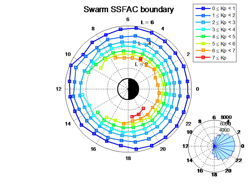
Figure 1: Mean boundary positions as a function of MLT at different levels of Kp (0-1,1-2,2-3,3-4,4-5,5-6,6-), and (bottom right) the MLT distribution of the boundary crossings.
Not only the boundary position, but also the boundary width is a function of Kp. The boundary gets narrower when geomagnetic activity increases. At low activity, the mean width is around 3 RE, but the scatter is large, while for Kp>6 it becomes narrower than 1 RE. The overwhelming majority of the boundary observations are made at relatively sharp boundaries, i.e. when the boundary width is lower than 3 RE.
For a given level of Kp, we model the observed boundary in L space by an eccentric circle. The position of a point P on the circle is given by its polar coordinates: Lmssfac and φ=2πMLT/24 as shown in Fig. 2. If the circle is centred at C(c,φc ) and has a radius R, Lmssfac can be derived for any MLT by applying the formula:
(1)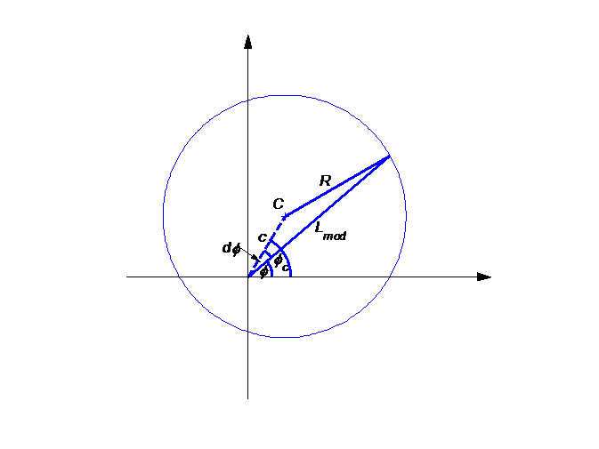
Figure 2: Sketch of the applied model at a fixed level of geomagnetic activity
Moreover, we suppose, that the position of C and the radius of the circle, R have a linear/quadratic dependence on Kp, respectively, that is
(2)where c0 and MLT0 define the position of the centre and R0 is the radius of the circle both Kp=0, while p1, p2, γc, γmlt are free model parameters. Based on 61512 boundary positions (here χ>90°) observed during the period Jan 1, 2014 - March 31, 2017, the following model parameters (with 95 % confidence bounds) were obtained:
The corresponding model is presented in Fig. 3 as dashed circular curves. The centres of the circulars hardly move with increasing Kp. From Kp = 0 to Kp = 6, it moves from MLTc=11.9, c= 0.18 RE to MLTc=12.9, c= 0.25 RE. The mean residuals (observation - model) in each bin are between -0.3-0.2 RE at all Kp levels between 1 and 6. At Kp = 0 the mean residuals are somewhat larger.
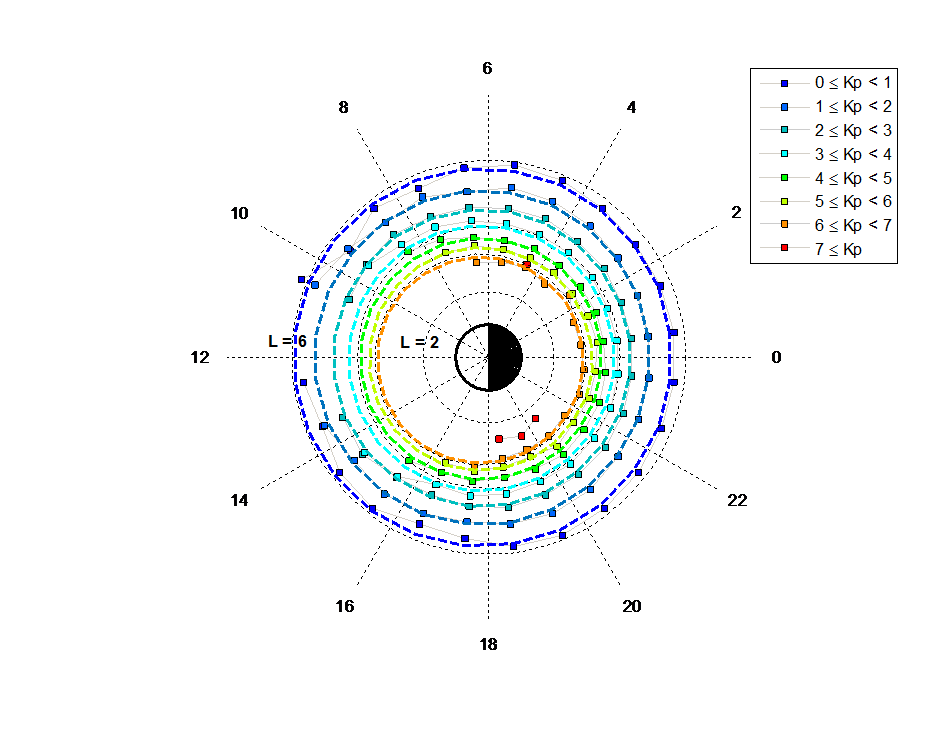
Figure 3: Empirical model of the inner SSFAC boundary. Only positions when χ>90° were used to derive the model.
The bulge model
The plasmasphere is well-known to have a dusk-side bulge and its distance at different MLTs can be quite different, controlled by the past variation of magnetospheric convection. On the contrary, the SSFAC boundary responds almost simultaneously at all MLTs (within about an hour) to changing conditions. The two boundaries are coupled only near midnight and in the early morning sector (Heilig and Lühr, 2017).
For calibration, we used NASA Van Allen Probes PP crossings obtained from in-situ electron density observations. We estimated the mean separation between the SSFAC boundary and the PP as a function of MLT. The calibration is based on 1762 Swarm crossings and the simultaneous (UT difference is less than ±1 h) VAP PP observations. The comparison revealed a clear bulge signature in the pre-midnight sector (19-01 h MLT) peaking at 21-22 h MLT. Elsewhere the SSFAC boundary is found typically poleward of the PP by ~0.5 R (Fig. 4). This result is very similar to the obtained differences between CHAMP and IMAGE observations (Heilig and Lühr, 2013). However, for individual cases the location of the boundaries can be very different. While the PP, due to its co-rotation with Earth and the localized erosion, is determined by the Kp evolution of the preceding days, the PP index responses within a few hours simultaneously at all MLTs.
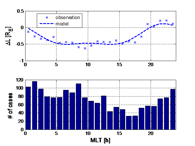
Figure 4: The bulge model
The 'bulge' model is deduced from the difference:
(3)Application of the model
The model derived in the previous section can be used in various ways. First, it can be used as a climatology model. When no boundary observations are available, Lmod can be calculated directly from MLT and Kp as inputs, then the bulge model value corresponding to the MLT in question has to be added. Using the model this way is similar to using any other statistical PP model:
(4)However, the strength of this model is that it can be used in synergy with PP indices, i.e. direct observations. If we have an observation of Lssfac=Lobs at a certain MLTobs and the geomagnetic activity given by the Kp index is known, we can, by combining the model (yielding the shape and the centre of the boundary) with the actual observation (providing the actual radius), estimate Lssfac at any other MLT. This is done by rescaling the size of the boundary based on the actual observation, while taking the average circular shape and the Kp-dependent centre position from the model:
(5)Moreover, since the Kp dependence of both c and MLTc is found to be very weak, we can regard them as constant, e.g. c=0.2 RE, MLTc=12 h, while
can be calculated from the model. Neglecting the Kp dependence of the centre position will cause less than 0.05 RE error.
Now Lmssfac at any MLT can be computed by the direct use of Eq. (1), but substituting R’ into R. The model PP position is
found again after adding the 'bulge' model.